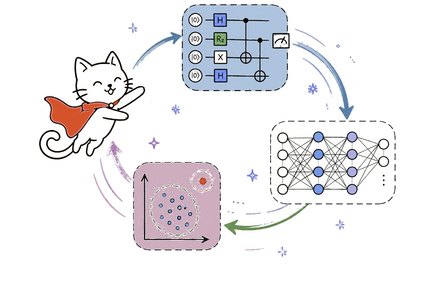
From Classical Machine Learning to Quantum Machine Learning

Machine learning is widely used for classification, prediction, pattern recognition, and anomaly detection ^{1 2}. Quantum machine learning, usually shortened to QML, asks whether quantum computers can contribute useful components to these learning workflows.

The answer is more nuanced than “quantum models are better.” On many small tasks with classical data, well-chosen classical models remain highly competitive, and the outcome of a comparison can depend strongly on preprocessing, model selection, and hyperparameter tuning ³. For this reason, near-term QML is often explored through hybrid quantum-classical workflows, in which a quantum circuit performs part of the computation while classical hardware handles the surrounding data processing and optimization ^{4 5}.

This post introduces the basic machine-learning workflow, explains where a quantum circuit can enter it, and gives an overview of the main approaches in QML. A follow-up post will focus specifically on quantum neural networks based on parameterized quantum circuits.

Classical machine learning in a nutshell

At a high level, machine learning is about learning useful patterns from data ².

A typical supervised-learning workflow can be summarized as:

Data → Model → Prediction → Loss → Optimizer → Updated Model

Its main components are:

• Input data: numerical features describing each sample.
• Model: a function with trainable parameters.
• Prediction: the model output for an input.
• Loss function: a measure of prediction error.
• Optimizer: an algorithm that updates the model parameters.
• Evaluation: a final test on data that was not used directly for training.

For example, a binary classifier receives an input vector and predicts whether it belongs to class 0 or class 1.

A neural network is one possible model. Its layers combine input values using trainable weights and biases:

$$ z = Wx + b, $$

where $x$ is the input, $W$ contains the weights, and $b$ contains the biases.

The result is then passed through a nonlinear activation function such as ReLU, sigmoid, or tanh. These nonlinearities allow a neural network to represent relationships that cannot be learned by stacking linear transformations alone ^{6 7}.

During training, the model produces a prediction, compares it with the correct target, and updates its parameters to reduce the loss.

A machine-learning model learns a mapping from inputs to outputs by adjusting trainable parameters.

Why classical baselines matter

A model is not automatically useful because it contains a quantum circuit. It must still be compared with classical methods that solve the same task under comparable conditions.

This is particularly important for small tutorial datasets. Logistic regression, support vector machines, tree-based models, and small neural networks may already perform very well. A benchmark by Bowles, Ahmed, and Schuld compared twelve common QML models on 160 binary-classification datasets and found that standard classical models generally performed better on the small-scale tasks studied ³.

A careful QML experiment should therefore ask:

• What does a simple classical baseline achieve?
• Are the data split and preprocessing identical?
• Were both model families tuned fairly?
• Which evaluation metric is appropriate?
• Does the quantum component add useful behavior or only complexity?

A tutorial does not need to demonstrate quantum advantage. Its purpose may instead be to explain the architecture, training loop, measurement process, and practical limitations of a hybrid model.

What is quantum machine learning?

Quantum machine learning combines concepts from quantum computing and machine learning ⁴.

In many QML applications, the input data is still classical. Numerical features are encoded into a quantum state or used as parameters of data-dependent quantum gates. A quantum circuit can then act as a feature map, similarity estimator, trainable model, or another component of the learning algorithm.

A simplified comparison is:

Classical ML:
input features → classical model → prediction

Quantum ML:
input features → quantum encoding → quantum circuit → measurement → classical output

A quantum circuit does not directly expose its quantum state as an ordinary numerical feature vector. Instead, classical information is extracted through measurement, for example as bitstring samples or estimated expectation values.

For a parameterized quantum model, the process may look like this:

input x
   ↓
data encoding
   ↓
quantum circuit U(x, θ)
   ↓
measurement
   ↓
measurement statistics
   ↓
numerical model output

On quantum hardware, an expectation value is generally estimated statistically from repeated measurement outcomes.

Main approaches in quantum machine learning

QML is a broad field, and its categories often overlap. Four commonly discussed approaches are variational quantum algorithms, quantum neural networks, quantum kernel methods, and quantum-inspired machine learning.

The first two typically involve trainable circuit parameters that are updated through an iterative quantum-classical optimization loop. Standard quantum kernel methods, by contrast, usually use a fixed quantum feature map and train the resulting kernel model classically.

Variational quantum algorithms

Variational quantum algorithms combine a parameterized quantum circuit (PQC) with a classical optimizer ⁵.

initial parameters
   ↓
parameterized quantum circuit
   ↓
measurement
   ↓
objective value
   ↓
classical optimizer
   ↓
updated circuit parameters
   ↺

The circuit contains adjustable parameters, such as rotation angles. After the circuit is executed and measured, a classical optimizer updates these parameters to reduce an objective function.

Examples include the variational quantum eigensolver (VQE), QAOA, and variational quantum classifiers ^{8 9}.

This hybrid pattern is not limited to machine learning. For example, IBM, Cleveland Clinic, and RIKEN recently combined parameterized quantum circuits with classical supercomputing resources in a large chemistry workflow ¹⁰. The study did not establish a clear quantum advantage, but it illustrated how quantum and classical resources can be integrated in scientific computing.

Quantum neural networks

Quantum neural networks are trainable quantum models inspired by neural-network learning. In near-term QML, the term often refers to models built from parameterized quantum circuits ^{11 12}.

classical input data
   ↓
quantum data encoding
   ↓
parameterized quantum circuit
   ↓
measurement
   ↓
prediction and loss
   ↓
classical optimizer
   ↓
updated model parameters
   ↺

The classical input data is encoded into a quantum state through data-dependent gates. The trainable circuit then transforms this state, while measurements provide numerical outputs that can be used to calculate predictions and a loss.

Like other variational approaches, PQC-based QNNs are usually trained through an iterative quantum-classical optimization loop.

Quantum kernel methods

Quantum kernel methods also begin by encoding classical input data into a quantum state ¹³. In this context, the encoding circuit is often called a quantum feature map because it maps the data into a quantum feature space in which similarities can be evaluated.

classical input data
   ↓
quantum data encoding / feature map
   ↓
quantum-state similarity estimation
   ↓
kernel matrix
   ↓
classical kernel model

The resulting quantum-computed kernel can be used by a classical algorithm such as a support vector machine.

Unlike variational quantum algorithms and PQC-based QNNs, a standard quantum kernel method usually does not update the parameters of the quantum feature map in an iterative quantum-classical training loop. Instead, the quantum circuit estimates similarities between encoded data points, while the resulting kernel model is trained classically.

Trainable quantum-kernel variants also exist, but the fixed-feature-map setting is the standard form introduced here.

Quantum-inspired machine learning

Quantum-inspired machine learning uses ideas associated with quantum systems while running entirely on classical hardware.

Tensor-network models are one example. They use structured mathematical representations developed for quantum many-body systems and apply them to machine-learning tasks ¹⁴. Unlike the approaches above, they do not require a quantum processor.

Conclusion

Quantum machine learning does not replace the familiar machine-learning workflow. It changes where and how part of the model is evaluated. Classical data preparation, optimization, and performance evaluation often remain essential, while a quantum circuit may act as a feature map, kernel component, or trainable model.

The main lesson is therefore not that quantum models are automatically superior, but that they introduce a different computational building block whose usefulness must be tested against strong classical baselines.

The next post narrows the discussion to one important model family: PQC-based quantum neural networks. It explains how they differ from classical neural networks, how measurement becomes part of the model output, and why their training loop is usually hybrid.