Vehicle Routing Problem with Quantum Annealing

The vehicle routing problem (VRP) is an NP-hard optimization problem in logistics. In our modern world, it is crucial to find a satisfactory solution in a short amount of time. In recent years, the approach of using quantum computing resources to solve the VRP has received increasing attention. As described in a review paper by Liu et al.¹, quantum annealing machines are most often used for optimization tasks in the logistics sector. We discussed the quantum annealing approach in a previous blog post and compared it to the gate-based framework for quantum computing.
In this blog post, we want to show how one can use quantum annealing to solve a VRP. We follow the approach proposed by Feld et al..² In a VRP, one has a fleet of vehicles, a list of customers, and a depot with their positions. The vehicles have a predefined capacity and the customers have a demand for products to be fulfilled. One has to decide which vehicle delivers the products to which customers. At the same time, the delivery time has to be minimized while the vehicle capacities must not be exceeded. Feld et al. divide the VRP into two phases: a clustering phase and a routing phase.
This post is part of the QUICS project, which is a collaboration of the GWDG, LUH, and the PTB. QUICS provides low-threshold access for SMEs to test use cases on different quantum hardware and software. All our code is available in our D-Wave Apptainer container. It is located in the directory /opt/notebooks/VRP/. You can inspect our current simulators here. Later, there will be the possibility of using quantum simulators within the HPC environment provided by the QUICS project.

The Clustering Phase

The clustering phase can be considered as a knapsack problem, where one packs differently sized objects into knapsacks with certain capacities, which are our vehicles here. Thus, for each cluster one vehicle is used. Feld et al. tackle this problem classically.
The first part of this phase is the cluster generation, which is structured as follows:

1. Choose the core stop of the cluster. Feld et al. suggest two different methods:
   a) choose the customer with the highest demand, or
   b) choose the customer which is the farthest away from the depot.
2. Calculate the geometric center of the cluster: $$CC(m_k) = \sum\limits_{i=0}^n \frac{v_i^x}{n}, \sum\limits_{i=0}^n \frac{v_i^y}{n}\, ,$$ where $m_k$ denotes the $k$-th cluster.
3. Select the customer with the shortest distance to the current geometric center of the cluster and add it to the cluster if its demand does not exceed the remaining capacity of the vehicle.
4. Recalculate $CC(m_k)$ and repeat (3.).
5. If the vehicle is full, finish the creation of this cluster and repeat from (1.) for the next cluster.

Secondly, the clusters have to be improved. For this, we choose a customer at random and compute its distance to the geometric center of the original cluster. Then we check in which other clusters the demand of the customer fits, and whether the customer is closer to one of these feasible clusters than to its original cluster. If this is the case, the customer is reassigned to the closest feasible cluster. This is repeated multiple times.

The Routing Phase

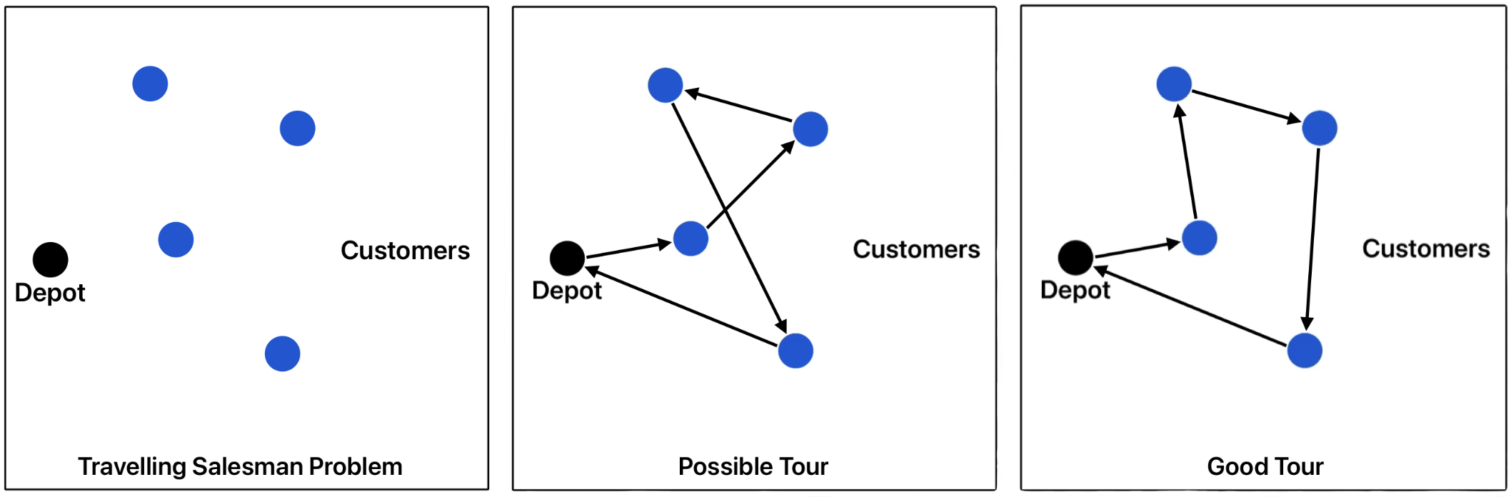
After the clustering phase, we have one traveling salesman problem (TSP) for each cluster. In the TSP there is only one vehicle (traveler) and the objective is to search for the optimal/shortest route. Such optimization problems can be solved using quantum annealing machines. To encode the problem for quantum annealing, we consider each TSP as a graph, where the customers and the depot are the vertices and the connections between all customers and the depot are the edges. The figure below illustrates a TSP together with two example tours. Both tours are feasible because each customer is visited exactly once. However, the tours do not have the same quality. The first tour has a length of $17.7$, and the second (good) tour has a length of $15.8$. This tour length³ is the objective of our example TSP to be minimized.

First, one has to define the Hamiltonian of this problem by combining the constraints and the objective function. For this, we define the binary variables $x_{uj}$, which are $1$ if customer $u$ is at position $j$ of the tour. The traveling times or distances between all customers can be written in a matrix $D$. Then, the objective function to be minimized can be written as

where $E$ is the set of all edges/connections between the customers, and $n$ is the number of customers. The first sum runs over all possible connections in the problem graph. In the second sum, the zeroth stop and the $n+1$-st stop are the depot. This ensures that shorter tours are favored by including a penalty $l\cdot B$ which increases if the length of the tour $l$ is larger.
We have three constraints in the TSP: the customer occurrence constraint, the tour position constraint, and the order-of-customers constraint. The customer occurrence constraint ensures that each customer occurs exactly once in the tour:

The tour position constraint ensures that each position in the tour is assigned to exactly one customer:

The order-of-customers constraint ensures that the order of customers is feasible:

This constraint only has to be included if not every customer is necessarily connected to every other customer. The full Hamiltonian of the problem is then $H = H_O + H_{C_1} + H_{C_2} + H_{C_3}$. The penalty parameters $B$ and $A$ have to be carefully chosen so that the constraints are satisfied, e.g. $0< B\cdot \max(D_{uv}) <A$.
The Hamiltonian description is equivalent to a QUBO problem. In our code, we use the QUBO formulation as the input to the quantum annealing machine. After applying the binomial formula and expanding the sums, one obtains the following implementation:

def objective_function(Q, B, x_var_index, travel_time_dict, customers, num_customers):
    """
    Q: QUBO matrix
    B: Penalty of the objective function
    x_var_index: Dictionary of the indices of the binary x variable
    travel_time_dict: contains all the travel times of all edges. Should be a dictionary with keys "uv"
    customers: The customer names / numbers of the TSP
    num_customers: Number of customers (not including the depot)
    """
    
    # Depot -> first customer:
    for u in customers:
        travel_time = travel_time_dict[("0", str(u))]
        idx = x_var_index[(u, 1)]
        Q[idx, idx] += B * travel_time

    # Customer -> customer transitions:
    for u in customers:
        for v in customers:
            if u != v:
                travel_time = travel_time_dict[(u, v)]
                for j in range(1, num_customers):
                    idx_1 = x_var_index[(u, j)]
                    idx_2 = x_var_index[(v, j + 1)]
                    Q[idx_1, idx_2] += B * travel_time

    # Last customer -> depot:
    for u in customers:
        travel_time = travel_time_dict[(str(u), "0")]
        idx = x_var_index[(u, num_customers)]
        Q[idx, idx] += B * travel_time
    return Q

def customer_occurance_constraint(Q, A, x_var_index, customers, num_customers):
    """
    Q: QUBO matrix
    A: Penalty of the constraint
    x_var_index: Dictionary of the indices of the binary x variable
    customers: The customer names / numbers of the TSP
    num_customers: Number of customers (not including the depot)
    """
    
    for u in customers:
        for j in range (1, num_customers+1):
            idx_1 = x_var_index[(u, j)]
            Q[idx_1, idx_1] -= A 

            for j_prime in range(1, num_customers+1):
                if j < j_prime:
                    idx_2 = x_var_index[(u, j_prime)]
                    Q[idx_1, idx_2] += 2*A 
    return Q

def tour_position_constraint(Q, A, x_var_index, customers, num_customers):
    """
    Q: QUBO matrix
    A: Penalty of the constraint
    x_var_index: Dictionary of the indices of the binary x variable
    customers: The customer names / numbers of the TSP
    num_customers: Number of customers (not including the depot)
    """
    
    for j in range(1, num_customers+1):
        for u in customers:
            idx_1 = x_var_index[(u, j)]
            Q[idx_1, idx_1] -= A 

            for u_prime in customers:
                if u < u_prime:
                    idx_2 = x_var_index[(u_prime, j)]
                    Q[idx_1, idx_2] += 2*A 
    return Q

Quantum Annealing Realization

To test the approach, we used the CMT1 dataset by Christofides et al. as an example. First, we create the clusters:

from create_clusters import cluster_generation, cluster_improvement

num_cluster_improve_iterations = 10000

initial_clusters = cluster_generation(customer_positions, customer_demand, depot_position, vehicle_capacity, use_demand_for_core_customer=False)
final_clusters = cluster_improvement(initial_clusters, num_cluster_improve_iterations, customer_positions, customer_demand, vehicle_capacity, depot_position)

The Python functions can be examined in our code. Then a TSP is solved for each cluster. We generate the QUBO matrix as described above and then create a binary quadratic model with the dimod library as the input to the simulator. We then use simulated annealing to solve the problem with the neal.sampler.SimulatedAnnealingSampler function.

import dimod
from neal.sampler import SimulatedAnnealingSampler

B = 1
for cluster_idx in list(final_clusters.keys()):
    customers = final_clusters[cluster_idx]
    num_customers = len(customers)
    
    ...
    
    A = 1000 * num_customers * B * max(travel_time_dict.values())
    
    # Get the QUBO matrix:
    Q = construct_qubo_matrix_for_TSP(A, B, customers, num_customers, travel_time_dict, set_of_edges)
    qubo = qubo_from_numpy(Q)

    # Create the BQM:
    bqm = dimod.BQM.from_qubo(qubo)
    
    # Use simulated annealing:
    sampler = SimulatedAnnealingSampler()
    response = sampler.sample(bqm, num_reads=3000, num_sweeps=6000)
    
    best_sample = response.first.sample 

If we execute this code, we get a total length of the tour between $1200$ and $1400$. The best known solution for the example is $524.61$. As you can see, with our experiment we do not get close to the best solution. The problem with our solution is that the solutions are not necessarily feasible. Some customers appear multiple times in the route. To achieve such high-quality solutions for these medium-sized problems, one needs to increase the number of reads (num_reads) and the number of sweeps (num_sweeps) in the simulator. However, this significantly increases the computation time. For our choice of parameters, the computation takes around $315,\text{s}$.
If we compare our timing results to those of Feld et al., we see that our computation takes much longer. Their computation on the D-Wave 2000Q model took only $15.792,\text{s}$ with the same dataset. Thus, the use of a real quantum annealer is significantly faster. Furthermore, their quantum annealing result is very close to the best-known solution.
In Feld et al., they also compare their calculation to a classical method, which took $1.474,\text{s}$. The quantum annealer takes much longer than the classical solution because of the computational overhead. This overhead is a result of the embedding of the problem onto the hardware graph. This is why embedding is a crucial part of quantum annealing research. If you look only at the actual computation time on the QPU, Feld et al.’s calculation takes only $0.110,\text{s}$.
To sum up, real quantum annealers can lead to sufficiently good solutions, even though their computational performance is not yet as good as that of classical methods. However, quantum annealers have great potential if the overhead time can be reduced. Moreover, annealing simulators don’t lead to sufficient results in a moderate amount of time. But such simulators can be useful for testing algorithms and code before using a real quantum annealer.